Constrained Optimization with Application to Synthetic Control Methods

Many of us who have worked in empirical economics research are familiar with quasi-experimental estimators for estimating causal effects, such as Difference-in-Differences, Regression Discontinuity Design, Instrumental Variables, and Propensity Score Matching. However, one innovative estimator that recently caught my eye during my master’s coursework was the Synthetic Control Method (SCM).

In this post, I will explore the computational aspects of SCM and provide some intuition (and math!) behind it in the backdrop of Pinotti’s (2015) study on the economic costs of organized crime. Using this empirical context, I will introduce and motivate the implementation of SCM, highlighting its application using Python’s rich scientific libraries. Specifically, I will draw on state-of-the-art quadratic programming solvers, including CVXOPT, OSQP, CPLEX, and scipy.optimize, to enhance the accuracy and reliability of SCM implementations.

Understanding the Synthetic Control Method

The Synthetic Control Method (SCM) was pioneered by Abadie and Gardeazabal (2003) in their estimation of the economic costs of terrorism in the Basque Country. It has since gained popularity for evaluating policy implications or interventions in empirical research, especially when dealing with observational data where randomized experiments are not feasible. The way it works is by constructing a ‘synthetic’ version of the treated unit by creating a weighted combination of control units that closely resemble the treated unit in the pre-treatment period. This ‘synthetic’ control then serves as a counterfactual to estimate what would have happened in the absence of the treatment.

Pinotti’s (2015) Study on the Economic Costs of Organized Crime

Pinotti’s 2015 study uses SCM to evaluate the economic impact of mafia activity on regional GDP in Italy. By exploiting the heterogeneous presence of mafia across Italian regions and the unique shocks in the 1970s that led to a rise in mafia activity in certain regions, Pinotti constructs a synthetic control to compare against the treated regions of Apulia and Basilicata. The study attributes a significant reduction in GDP per capita to the presence of organized crime.

The two idiosyncratic shocks, namely the closure of the Tangier port and the earthquake in Basilicata, not only ushered in a sharp rise in mafia activity in Apulia and Basilicata, but these events can also be considered to be plausibly independent of these regions’ social and economic conditions at the time. This allows for a subdivision of the Italian regions into treated, control, and excluded categories as follows:

• Treated: Apulia, Basilicata
• Control: Abruzzo, Molise, Sardinia, Piedmont, Aosta Valley, Lombardy, Trentino Alto Adige, Veneto, Friuli Venezia Giulia, Liguria, Emilia Romagna, Tuscany, Umbria, Marche, Lazio
• Excluded: Sicily, Campania, Calabria

The ‘Treated’ units are the regions that were affected by these events and as a result witnessed a rise in mafia presence. I follow Pinotti’s (2015) methodology of using an aggregated composite of these two regions that combines their outcome and predictor variables into one ‘treated’ region.

The ‘Control’ units are the unaffected regions and therefore comprise the ‘donor pool’ from which to construct a synthetic control. The core idea is to assign weights to each unit in the donor pool so that the resulting synthetic control mimics the pre-1970s economic conditions of the treatment group as closely as possible in the matching period (1951-1960). The synthetic control unit can then be used as a counterfactual scenario to the treatment unit for the post-treatment period.

Technical Breakdown

Now for some math. To formally define the SCM used as part of the methodology, let $ y_t $ be an outcome of interest at time $t$ which depends on the presence of organized crime. Each region will have outcome $y^1$ if exposed to organized crime, and $y^0$ otherwise:

where $c_t$ is a binary indicator for the presence of organized crime in the region. Of course, in reality we only observe one of the two potential outcomes in a given year, but the treatment effect we are interested in is given by $\beta_t=y^1_t-y^0_t$.

The synthetic control method allows us to overcome this issue. The estimator will compare the actual outcome in the treatment group to a weighted average of the units in the control group.

where $w_t$ are the weights associated with each region in the control group $I$.

The question is then how to choose the weights. The approach in Abadie et al. (2021) is to optimize the weights with the aim of minimizing the distance between the treatment and control group in the pre-treatment period, that is, before the occurence of the two pivotal events that induced the mafia presence. So the optimal vector of weights $W^*(V)$ that minimizes the square distance between the two groups is:

where $x$ and $x^0_i$ is the $(K\times 1)$ vector of predictors and $V$ is the $(K\times K)$ diagonal matrix with non-negative entries measuring the relative importance of each predictor in the model.

Therefore, we choose $V$, the matrix of predictor weights, with the aim of minimizing

Finally, the mean square error is minimized over 1951-1960 which is the author’s pre-treatment period.

Implementing SCM with Python: Simplified Optimization

The first step in implementing SCM involves setting up a simplified optimization problem where predictor weights are initially assumed to be equal. This helps in understanding the basic mechanics of SCM and provides a baseline for further optimization. Using Python’s CVXPY package, I set up a convex optimization problem to minimize the distance between the treated unit and the synthetic control in the pre-treatment period.

The objective function is given by:

subject to

The code for this setup is as follows:

def w_optimize(v_diag, solver=cp.ECOS):
    V = np.zeros(shape=(8, 8))
    np.fill_diagonal(V, v_diag)
    
    W = cp.Variable((15, 1), nonneg=True)  # Creates a 15x1 positive nonnegative variable
    objective_function = cp.Minimize(cp.norm(V @ (X1 - X0 @ W)))
    objective_constraints = [cp.sum(W) == 1]
    objective_problem = cp.Problem(objective_function, objective_constraints)
    objective_solution = objective_problem.solve(solver, verbose=False)
    
    return W.value, objective_problem.constraints[0

].violation(), objective_solution

w_basic = cvxpy_basic_solution(control_units, X0, X1)

Optimization with Addition of Predictor Importance

To account for the heterogeneity in the effect of the 8 predictor variables on the outcomes $Y$ (GDP per capita in Pinotti’s case), Abadie and Gardeazabal (2003) proposed augmenting the optimization objective with a $(k × k)$ diagonal matrix $V$, such that the diagonal elements are weights indicating the relative importance of each of the predictors. The problem becomes,

(3) \(W^*(V)={\operatorname{arg}}\min _{W \in \mathcal{W}}\left(X_{1}-X_{0} W\right)' V\left(X_{1}-X_{0} W\right)\)

Equation (3) is the ‘inner’ optimization objective with the goal of minimizing the distance between the predictor values of the $J$ donor units, the $(k × J)$ matrix $X_{0}$, and those of the treated unit, the $(k × 1)$ vector $X_{1}$ given predictor importance weights $V$.

(4) \(V={\operatorname{arg}}\min _{V \in \mathcal{V}}\left(Z_{1}-Z_{0} W^*(V)\right)' \left(Z_{1}-Z_{0} W^*(V)\right)\)

Equation (4) is the ‘outer’ optimization objective to find the optimal diagonal matrix of predictor weights $V$ that minimize the RMSPE of the outcome variable $Y$ in the pre-intervetion period (Becker and Klößner, 2018:4). So the diagonal elements themselves become part of the optimization steps in the calculation of the synthetic controls.

Moreover, they are subject to their own constraints, namely that $V$ is a subset of all positive semi-definite diagonal matrices, such that the diagonal elements sum to one (Malo et al.,2020:4):

Nested Optimization

To improve the optimization function, I draw on insights from recent popular implementations of SCM, such as Hainmueller’s Synth package in R and its adaptations to MATLAB and STATA, as well as the more recent R/MSCMT package of Becker and Klößner (2018). Although these packages do not have adaptations for Python, I draw on some of their main insights and adapt them.

My particular focus is the R/MSCMT package since it offers a generalization of the SCM that addresses the instabilities and shortfalls of existing implementations. This package has several optimization algorithms, including one that uses a combination of outer optimization via Differential Evolution and inner optimization via DWNNLS (Weighted Non-Negative Least Squares). This corresponds to the default option ‘DEoptC’ in the call to R/MSCMT’s solver. The Fortran implementation of the WNNLS algorithm was presented by Hanson and Haskell (1982) and was later adapted to R in the package limSolve (Becker and Klößner, 2018). WNNLS is a reliable and fast inner optimizer for the nested optimization problem of SCM, which the authors of R/MSCMT enhance with a further speed boost by using Fortran calls to WNNLS in a C-implementation.

I adapt some of these ideas using Python’s existing libraries. Differential Evolution for the outer optimization is available via the scipy.optimize library. However, Python currently does not have a wrapper for WNNLS. Therefore, I instead use ECOS via CVXPY as the default solver. To add some flexibility to this approach, I insert the optimization method into a configurable function with a built-in data-preparation tool.

Here is the code for the final nested optimization function:

def SCM_v1(data, unit_identifier, time_identifier, matching_period, treat_unit, control_units, outcome_variable, predictor_variables, reps=1, solver=cp.ECOS, seed=1):
    """
    Nested Optimization
    """
    
    X0, X1, Z0, Z1 = data_prep(data, unit_identifier, time_identifier, matching_period, treat_unit, control_units, outcome_variable, predictor_variables)
    
    # Inner optimization
    def w_optimize(v):
        V = np.zeros(shape=(len(predictor_variables), len(predictor_variables)))
        np.fill_diagonal(V, v)
        W = cp.Variable((len(control_units), 1), nonneg=True)
        objective_function = cp.Minimize(cp.norm(V @ (X1 - X0 @ W)))
        objective_constraints = [cp.sum(W) == 1]
        objective_problem = cp.Problem(objective_function, objective_constraints)
        objective_solution = objective_problem.solve(solver)
        return W.value
    
    # Outer optimization
    def vmin(v): 
        v = v.reshape(len(predictor_variables), 1)
        W = w_optimize(v)
        return ((Z1 - Z0 @ W).T @ (Z1 - Z0 @ W)).ravel()
    
    # Constraint on the sum of predictor weights
    def constr_f(v):
        return float(np.sum(v))

    # Setting Hessian to zero as advised by Differential Evolution to improve performance
    def constr_hess(x, v):
        v = len(predictor_variables)
        return np.zeros([v, v])

    # Must also set Jacobian to zero when setting Hessian to avoid errors
    def constr_jac(v):
        v = len(predictor_variables)
        return np.ones(v)
    
    def RMSPE_f(w):  # RMSPE Calculator
        return np.sqrt(np.mean((w.T @ Z0.T - Z1.T) ** 2))
    
    # Differential Evolution optimizes the outer objective function vmin()
    def v_optimize(i):
        bounds = [(0, 1)] * len(predictor_variables)
        nlc = NonlinearConstraint(constr_f, 1, 1, constr_jac, constr_hess)
        result = differential_evolution(vmin, bounds, constraints=(nlc), seed=i)
        v_estim = result.x.reshape(len(predictor_variables), 1)  
        return v_estim
    
    # Function that brings it all together step-by-step
    def h(x):
        v_estim1 = v_optimize(x)  # Finding v* once Differential Evolution converges at default tolerance
        w_estim1 = w_optimize(v_estim1)  # Finding w*(v*)
        prediction_error = RMSPE_f(w_estim1)
        output_vec = [prediction_error, v_estim1, w_estim1]
        return output_vec

    iterations = []
    iterations = Parallel(n_jobs=-1)(delayed(h)(x) for x in list(range(seed, reps + seed)))  # Seed for replicability
                                                                                            # Can increase repetitions
    solution_frame = pd.DataFrame(iterations)
    solution_frame.columns = ['Error', 'Relative Importance', 'Weights']
    solution_frame = solution_frame.sort_values(by='Error', ascending=True)

    w_nested = solution_frame.iloc[0][2]
    v_nested = solution_frame.iloc[0][1].T[0]
    
    output = [solution_frame, w_nested, v_nested, RMSPE_f(w_nested)]  # [All repetitions, W*, V*, RMSPE]
    
    return output

# Setting SCM function arguments as in Pinotti (2015)
unit_identifier = 'reg'
time_identifier = 'year'
matching_period = list(range(1951, 1961))
treat_unit = 21
control_units = [1, 2, 3, 4, 5, 6, 7, 8, 9, 10, 11, 12, 13, 14, 20]
outcome_variable = ['gdppercap']
predictor_variables = ['gdppercap', 'invrate', 'shvain', 'shvaag', 'shvams', 'shvanms', 'shskill', 'density']
entire_period = list(range(1951, 2008))

output_object = SCM_v1(data, unit_identifier, time_identifier, matching_period, treat_unit, control_units, outcome_variable, predictor_variables)

w_nested = output_object[1]
v_nested = output_object[2]

SCM_print(data, output_object, w_pinotti, Z1, Z0)

The SCM implementation has replicated the weights obtained by Pinotti’s STATA implementation in a faster and more reliable manner than the previous approach. As a result, the outer objective function values are approximately equal.

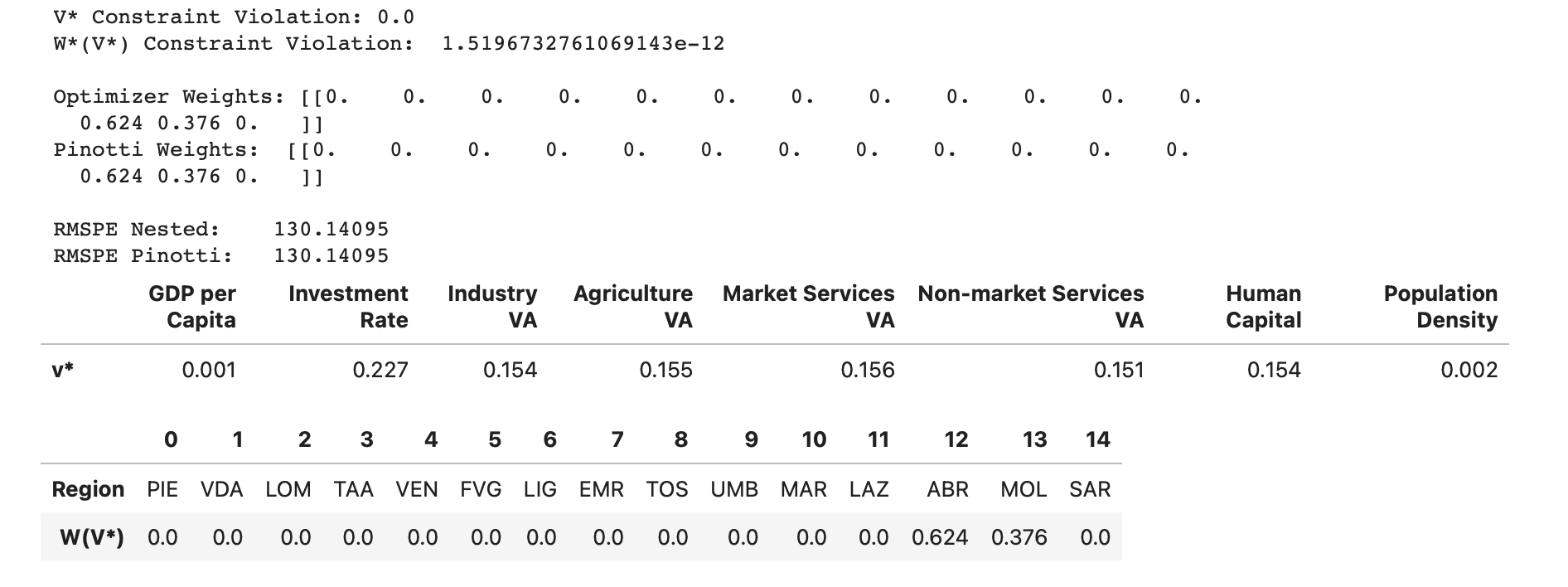
I also observe that the corresponding $( V )$ allocates higher weights to investment rate, industry share of value added, and non-market services share of value added. The relatively large weight on the investment rate is especially unsurprising since, from an economic standpoint, one would expect investment in an economy to be highly correlated with output as seen in standard growth models in macroeconomics.

Conclusions

The Synthetic Control Method is a valuable tool for causal inference in empirical research, offering a rigorous way to construct counterfactuals in observational studies. By leveraging Python’s rich scientific libraries and advanced optimization techniques, we can enhance the accuracy and reliability of SCM implementations. This project not only replicates Pinotti’s findings on the economic impact of organized crime but also provides a robust framework for applying SCM to various empirical contexts.