The best part about joining the research team Wharton was the exposure to some of the most innovative methods being deployed at the current frontiers of economic analysis in energy and environment. That applied also to my first week in the Business Economics and Public Policy department. For my very first project, I had the opportunity to dive head-first into a challenging geospatial economics project. For this project, my principal investigator was seeking to answer the question: to what extent have EU land protection policies actually contributed to the continent’s greening and biodiversity?
Although I had previously worked with geospatial data, namely through my application of Convolutional Neural Networks to satellite images for poverty prediction in Malawi, I ran into several fun challenges in this project simply because of the scale and richness of data involved. This included constructing datasets to the tune of ~100 million data points in total, which required building up my technical skills in big data analytics and setting up effective workflows for handling large datasets through automation. Lots of it. Because of the highly granular of geospatial data, this post will provide an inside scoop to anyone looking to get started with geospatial analysis and help save time by avoiding some of the pitfalls I ran into.
Project Overview
Just for a bit of context - the issue of land protection in the face of rapid deforestation and urban sprawl has been a long-standing one, gaining traction at COP15 with Europe pledging to protect 30% of its land by 2030. A more recent extension of this was the Kunming-Montreal Global Biodiversity Framework. This pact was signed by several nations with the aim of protecting 30% of the planet’s land and water by 2030. It’s a bold move to curb the alarming rate at which we’re losing forest cover and diverse species. Europe, not one to lag behind, had by then already safeguarded 26 percent of its landscapes and waterways.
To quantitatively assess the effectiveness of Europe’s circa 26% protected land in bolstering the region’s nature reserves, we needed highly granular datasets for analysis that would:
- Tell us the land protection status of a given chunk of land.
- Measure the greenning of that land overtime.
- Provide other geo-physical land characteristics about the land.
Data Collection
The raw data for this project was obtained from several sources. For example, our primary measure of greenness, Normalized Difference in Vegetation Index (NDVI), was sourced from Google Earth Engine. In addition, key agronomic data such as soil suitability was received from ESDAC and Europe’s protected sites coverage from EEA. The national boundary shapefiles that were the starting point of our datasets were obtained from Eurostat. Most these data were freely accessible from the relevant online websites (although some sources like ESDAC had a request and approval process) so I think anyone looking to follow along can readily do so.
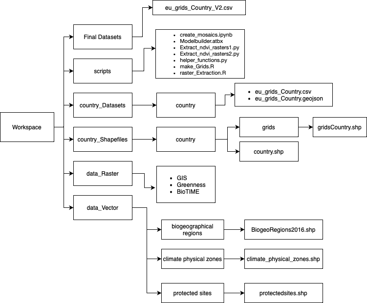
Big Data Tip #1: Being super-organized with geospatial data.
Unlike raw data in a typical .csv or similar format which can be housed in a simple two-folder set-up (raw and processed), geospatial data can quickly become difficult to keep track of as its processed down multiple layers of a data pipeline, especially when dealing with data from several sources, with each requiring its own processing in ArcGIS/R.
As a simple example, at the very basic level I started with a block of Eurostat national boundaries for Scandinavia in shapefile format. The raw shapefile had to be split up into the separate countries manually in ArcGIS, then those separate components had to be stored locally. Further down the data pipeline, the shapefile was converted from shapefile format to. geojson and then finally .csv. All these raw, intermediate, and final data can be easily misplaced especially when dealing with several countries. This is especially troublesome when you want to head back to a previous step and change some processing steps, but the original file cannot be located!
One effective way to pre-emptively mitigate against this is to establish an organized workflow from the beginning. Along with this, establishing a file naming convention such as _raw, _clean, _final denoting the various stages of processing of geospatial data. And finally, maintaining thorough documentation at each step, detailing what was done. As an example, I established the following folder structure for this project (feel free to re-purpose for your own needs):
Data Challenges
We defined a unit of observation in the datasets as a 300 meters by 300 meters grid cell that is constant across time. Grid cells divide European country’s geographic areas into evenly spaced areas with corners given by latitude and longitude coordinates, and each grid cell is uniquely identified by the combination of its centroid x and y coordinate. These grids were generated for 32 countries listed in the CDDA database.
More generally, the process of building geospatial datasets for European countries on these grids was… an interesting one. Our primary measure of greenness, Normalized Difference in Vegetation Index (NDVI), was constructed from Landsat images from 1985 through 2019. However, due to presence of dense cloud cover in the months, we constructed an algorithm that used a rolling window to select images that captured the clearest view of a given country’s vegetation.
Moreover, mapping spatial vector data (mostly categorical data such as climate zones and bio-geographical regions) in ArcGIS Pro was tediously slow when done manually for larger country’s with several million 300m x 300m grids cells. So instead doing these manually for 32 countries, I created an ArcGIS toolbox to automate this at the country-level and let it run while I worked on other tasks. Which leads me to my second tip.
Big Data Tip #2: Spending time to save time (and headaches) by automating workflows.
An adage I learned from my Effective Programming for Economists course at Uni Bonn was that, if a particular line of code has to be run even more than once, define a function and use ‘lapply’ or ‘for’ loop to automate it away. Of course, this may not always be necessary, but it certainly helped me with constructing these massive datasets. I exemplify these with two use cases:
1) ArcGIS Pro Toolbox and ArcPy
It is likely that if you’ve worked with geospatial data before you may be familiar with this software. Given my programming-heavy background, I was a bit surprised that many of the online tutorials and guidance I got on using ArcGIS were framed with considerable focus of manual clicking, dragging, and general weaseling through countless menus.
This seemed problematic for a couple of reasons: first, obviously due to human error - there is always a chance when doing spatial computations manually that one might select the wrong attribute for a spatial join, set the wrong coordinate reference system, or forget to select certain parameters. Second, what if I need to apply a similar set of spatial processes across multiple countries? This would not only be very time-consuming but also magnify the risk of the previous point.
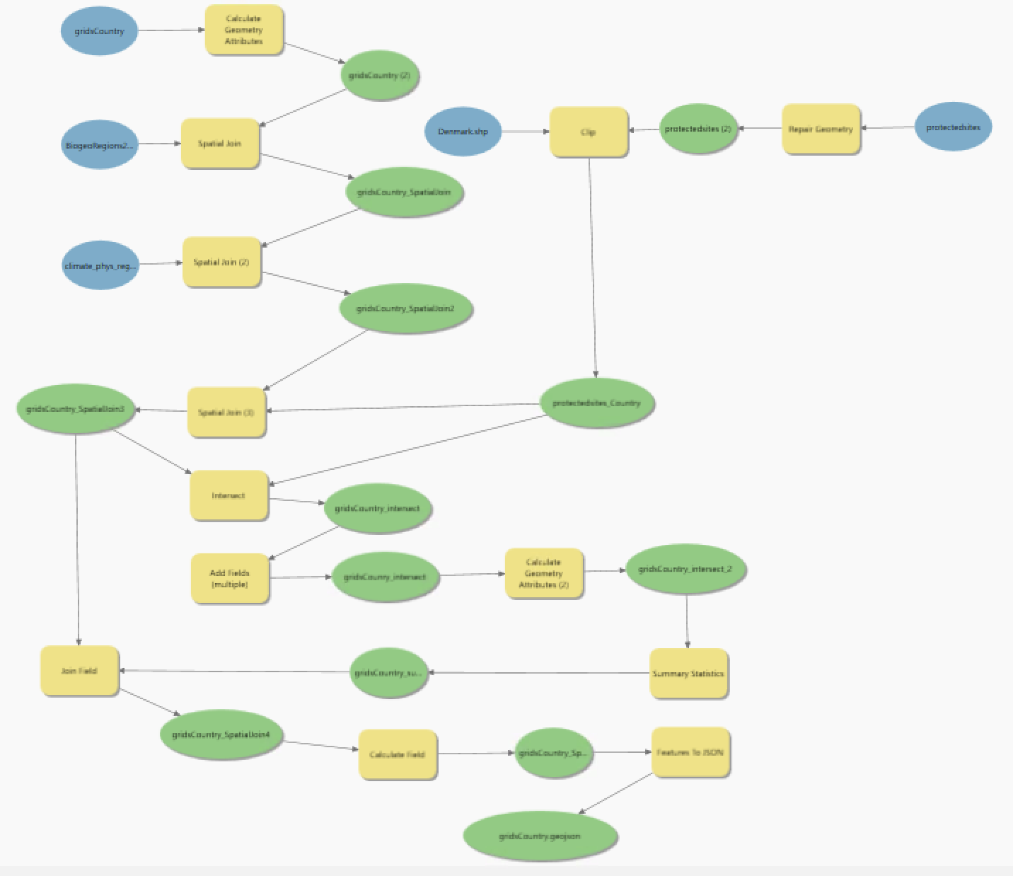
The trick I learned here is to automate series of spatial processes with the convenient toolbox in ArcGIS or alternatively to write the commands in ArcPy. The Modelbuilder tool in ArcGIS allows you to create DAGs (Directed Acyclic Graphs) to represent geoprocessing workflows and tools. I found these to be a visually appealing and logical way to show the processing steps applied to a country’s shapefile, ensuring the ordering of the steps made sense, for example, by repairing the original protected sites shapefile, repairing it to fix topology errors, and then spatially joining it to the country shapefile join. These DAGs also conveniently double as documentation, which is an added benefit.
2) Functions for Raster Processing in R
During my database construction, I ran into several multi-band rasters which captured some geo-physical process overtime. For example. we wanted to include rainfall history for every grid cell from 1985 through 2019, and so this involved extracting the corresponding band from the rainfall raster. This is a tiny snippet of what I came across in an initial build of the raster extraction script:
rainfall1985 <- raster(“C:/Users/Tristan/Desktop/ForestTransition/rain/rain_1985.tif”) rainfall1986 <- raster(“C:/Users/Tristan/Desktop/ForestTransition/rain/rain_1985.tif”) rainfall1987 <- raster(“C:/Users/Tristan/Desktop/ForestTransition/rain/rain_1987.tif”)
It is easy to spot the mistake now (spoiler - the rain_1985 raster is accidentally being mapped onto the variable for 1986). But, at the time, I spent a lot of hours debugging an issue in the analysis which was traced down to this line buried within some 1600 other lines of code. The best practice to avoid this kind of situation and possibility of human error would be to apply a loop or function that does away with repeated lines of code. Here’s what I changed this to:
for (year in rainfall_years) { raster_path <- paste0(“../data_Raster/GIS/eu_rain_ERA_5/rain_”, year, “.tif”) raster_name <- paste0(“rainfall”, year) assign(raster_name, raster(raster_path)) country_grids[,paste0(“rain”,year)] <- exact_extract(eval(as.symbol(paste0(“rainfall”,year))),country_grids,’mean’) }
This alternative condensed 25 lines of code into a simple loop and avoided any hard-coding that might be prone to human error. I highly recommend adopting such practices in your own workflow when dealing with multi-band rasters or generally with rasters that require repetitive processing steps (which in this case is just a raster being extracted to a country’s grid)
Geospatial Data Construction
There were several scripts involved in my data pipeline. Although I won’t push into too much detail here (I defer to the project’s replication package, which offers a thorough step-by-step guide), I would like to point to one script in particular which is the raster extraction script. It is likely that if you’re working with geospatial data, you may have wanted to map a raster’s value onto a shapefile (essentially converting a TIFF file into .csv columns). As it turned out, this ended up being the most challenging part of data pipeline.
The reason for this is that the processes of extracting raster data (data that utilizes grid-based structure for storing numerical values, mostly continuous phenomenon like NDVI, rainfall as outline previously etc.) to the country datasets was computationally intensive, even for relatively smaller countries like Switzerland. Eventually, I got fed up of R’s “vector memory exhausted” errors when running this on my computer and decided to push the process to a better computer; to the “Cluster” - Wharton’s High Performance Computing (HPC) facility.
Big Data Tip #3; Leveraging High Performance Computing
The use of Wharton’s HPC drastically changed my project’s timeline since tasks instantly went from taking several days for the raster extraction of a single country to just a few hours. However, in case you don’t have access to HPC, I think some of the concepts here can still help in terms of getting the most of out existing resources:
1) Array Jobs: Typically, multi-core processing using the ‘parallel’ library in R with some combination of ‘mclapply’ would’ve done the job for a big chunk of the computationally intensive Monte Carlo simulation I did during my masters thesis research. However, for handling geospatial data, I didn’t just need more processing power, but also greater access to RAM. I achieved this by splitting up by raster extraction into 12 parts - since each part was independent of each other (that is the output of any given part was not an input for any other) and running each of them simultaneously using Wharton HPC’s array job functionality. This conveniently allowed me speed up my workflow by a factor 4. The only caveat was that I had to merge the output from the individual parts back together into one collective dataset. But this merging itself took only a few minutes.
2) UNIX Command Line: I severely disliked using UNIX command line tools during my undergraduate ‘Intro to Computer Science class’ at Emory, but realized when working with HPC on geospatial data that it can greatly enhance your efficiency when working with large datasets, even without access to high-performance computing resources. For example:
a) File Manipulation: UNIX commands like grep, awk, and sed are powerful for searching, filtering, and transforming data. For example, you can use grep to extract specific lines from text files, awk to perform complex text processing tasks, and sed to search and replace text patterns (i.e. making corrections that applies to several R scripts becomes quick and easy)
b) Batch Processing: You can use shell scripting to automate repetitive tasks and perform batch processing on multiple files. By writing simple shell scripts, you can chain together UNIX commands to create powerful data processing pipelines. Just like with this project, I created a batch pipeline at multiple levels: running a batch of R scripts, for a batch of countries, then merging all the individual components for each country into a country dataset.
d) Remote Access: If you’re working on a remote server or cloud platform, SSH (Secure Shell) allows you to securely connect to the remote machine and execute commands remotely. This can be useful for running computationally intensive tasks on a server with more resources than your local machine, with the benefit of being able to access it anywhere.
Geospatial Analysis for the Future
The 32 final datasets created as part of this project corresponded to our sample of 32 EU countries contained 172 variables on forest cover, agronomic characteristics, and spatial information. To the tune of ~100 million data points in total. After employing a staggered difference-in-differences design using these data, we found that the protected area policies did not have a meaningful impact on either vegetation cover or economic activity measured by nightlights across various countries and time periods. The study suggested that land selected for protection was not under immediate threat, hence the limited impact.
This project underscored that the role of comprehensive and granular data analysis is crucial in evaluating the real-world impact of policy measures. Despite the ambitious targets set by EU policies, our findings highlight the importance of not just protecting more land but focusing on areas that truly require intervention to prevent degradation. It also serves as a reminder of the potential disconnect between policy goals and on-the-ground outcomes, urging a more strategic approach that aligns conservation efforts with ecological needs and economic realities.
In conclusion, while the initial results may seem disheartening, they provide valuable insights for refining conservation strategies. Moreover, this project underscored the importance of leveraging massive amounts of high-resolution geospatial data to understand the real-world impacts of environmental policies. By employing advanced data management and analysis techniques, such as cloud computing and high-performance computing clusters, we were able to handle and analyze approximately 100 million data points efficiently. This approach not only facilitated a deeper understanding of policy effectiveness but also highlighted the critical role of strategic data analysis in environmental conservation efforts.